In [1]:
using Pkg
Pkg.activate(@__DIR__)
 Activating environment at `~/Mathematics/Research/MATH+_approximate+convex+hulls/polymake-icms/notebooks/Project.toml`
In [2]:
Pkg.status()
Status `~/Mathematics/Research/MATH+_approximate+convex+hulls/polymake-icms/notebooks/Project.toml`
  [f213a82b] HomotopyContinuation v1.4.4
  [55ecb840] ImplicitPlots v0.1.3
  [91a5bcdd] Plots v1.0.14
  [d720cf60] Polymake v0.4.2

Interactive polyhedral computation with Jupyter+Julia+

by Marek Kaluba (TU Berlin, AMU Poznań), Sascha Timme (TU Berlin), Benjamin Lorenz (TU Berlin)

Polymake.jl

Installation

In [3]:
import Pkg
Pkg.add("Polymake")
   Updating registry at `~/.julia/registries/General`
    
   Updating git-repo `https://github.com/JuliaRegistries/General.git`

  Resolving package versions...
   Updating `~/Mathematics/Research/MATH+_approximate+convex+hulls/polymake-icms/notebooks/Project.toml`
 [no changes]
   Updating `~/Mathematics/Research/MATH+_approximate+convex+hulls/polymake-icms/notebooks/Manifest.toml`
 [no changes]
In [4]:
Pkg.status()
Status `~/Mathematics/Research/MATH+_approximate+convex+hulls/polymake-icms/notebooks/Project.toml`
  [f213a82b] HomotopyContinuation v1.4.4
  [55ecb840] ImplicitPlots v0.1.3
  [91a5bcdd] Plots v1.0.14
  [d720cf60] Polymake v0.4.2
In [5]:
using Polymake
polymake version 4.0
Copyright (c) 1997-2020
Ewgenij Gawrilow, Michael Joswig, and the polymake team
Technische Universität Berlin, Germany
https://polymake.org

This is free software licensed under GPL; see the source for copying conditions.
There is NO warranty; not even for MERCHANTABILITY or FITNESS FOR A PARTICULAR PURPOSE.

Functionality

The polymake objects a user encounters can roughly be divided in three classes

  • big objects (e.g., cones, polytopes, simplicial complexes),
  • small objects (e.g., matrices, polynomials, tropical numbers),
  • user functions

All* are easily accessible through Polymake.jl.

Big objects

Broadly speaking, big objects correspond to mathematical concepts with well defined semantics.

In [6]:
p = polytope.Polytope(POINTS=[1 1 2; 1 3 4])
Out[6]:
type
Polytope
POINTS
1 1 2
1 3 4

Big objects can be e queried for their properties (they are only computed when queried for the first time)

In [7]:
p.VERTICES
polymake: used package cdd
  cddlib
  Implementation of the double description method of Motzkin et al.
  Copyright by Komei Fukuda.
  http://www-oldurls.inf.ethz.ch/personal/fukudak/cdd_home/

Out[7]:
pm::Matrix<pm::Rational>
1 1 2
1 3 4
In [8]:
p
Out[8]:
type
Polytope
CONE_AMBIENT_DIM
3
CONE_DIM
2
FEASIBLE
true
FULL_DIM
false
LINEALITY_SPACE
N_POINTS
2
POINTED
true
POINTS
1 1 2
1 3 4
VERTICES
1 1 2
1 3 4

The documentation is also accessible from the package (though still in perl syntax):

In [9]:
?polytope.rand_sphere
Out[9]:
rand_sphere<Num>(d, n; Options) -> Polytope<Rational>

 Produce a rational d-dimensional polytope with n random vertices
 approximately uniformly distributed on the unit sphere.

Type Parameters:
  Num can be AccurateFloat (the default) or Rational
    With AccurateFloat the distribution should be closer to uniform,
    but the vertices will not exactly be on the sphere.
    With Rational the vertices are guaranteed to be on the unit sphere,
    at the expense of both uniformity and log-height of points.

Arguments:
  Int d the dimension of sphere
  Int n the number of random vertices

Options: 
  seed => Int controls the outcome of the random number generator;
    fixing a seed number guarantees the same outcome. 
  precision => Int Number of bits for MPFR sphere approximation

Returns Polytope<Rational> 
In [10]:
p = @pm polytope.rand_sphere{AccurateFloat}(3, 10)
Out[10]:
type
Polytope
description
Random spherical polytope of dimension 3; seed=10844047612566873288; precision=default
BOUNDED
true
CONE_AMBIENT_DIM
4
POINTS
1 -3582977214079311/36028797018963968 6367130133661991/9007199254740992 -3153844258136881/4503599627370496
1 2954143123681545/9007199254740992 -4190365832203919/4503599627370496 1471738288080989/9007199254740992
1 6209462095132723/9007199254740992 4096010470992269/9007199254740992 -5078869670038631/9007199254740992
1 -4757957716205513/18014398509481984 5351758314602071/18014398509481984 -1033121549773645/1125899906842624
1 -2465797302842971/9007199254740992 7802901811304839/9007199254740992 -1881768144527553/4503599627370496
1 1792380333301801/18014398509481984 -2977082379873531/9007199254740992 -8453606455427853/9007199254740992
1 9003973105085525/18014398509481984 -5250323055028577/9007199254740992 180320524391329/281474976710656
1 -742295239609249/1125899906842624 6769229861376577/9007199254740992 6637454368895073/288230376151711744
1 2554350309477553/9007199254740992 4312083045762249/4503599627370496 7651482669436381/144115188075855872
1 5928218345089213/18014398509481984 -121381931680819/140737488355328 -865844199072253/2251799813685248

Small objects

Small objects correspond to types or data structures which are implemented in C++.

In [11]:
p.VERTICES
Out[11]:
pm::Matrix<pm::Rational>
1 -3582977214079311/36028797018963968 6367130133661991/9007199254740992 -3153844258136881/4503599627370496
1 2954143123681545/9007199254740992 -4190365832203919/4503599627370496 1471738288080989/9007199254740992
1 6209462095132723/9007199254740992 4096010470992269/9007199254740992 -5078869670038631/9007199254740992
1 -4757957716205513/18014398509481984 5351758314602071/18014398509481984 -1033121549773645/1125899906842624
1 -2465797302842971/9007199254740992 7802901811304839/9007199254740992 -1881768144527553/4503599627370496
1 1792380333301801/18014398509481984 -2977082379873531/9007199254740992 -8453606455427853/9007199254740992
1 9003973105085525/18014398509481984 -5250323055028577/9007199254740992 180320524391329/281474976710656
1 -742295239609249/1125899906842624 6769229861376577/9007199254740992 6637454368895073/288230376151711744
1 2554350309477553/9007199254740992 4312083045762249/4503599627370496 7651482669436381/144115188075855872
1 5928218345089213/18014398509481984 -121381931680819/140737488355328 -865844199072253/2251799813685248
In [12]:
dump(p.VERTICES)
Polymake.MatrixAllocated{Polymake.Rational}
  cpp_object: Ptr{Nothing} @0x000000000565e630

Small objects follow the Julia semantics and expected behaviour as closely as possible

In [13]:
# Indexing works
p.VERTICES[1, :]
Out[13]:
pm::Vector<pm::Rational>
1 -3582977214079311/36028797018963968 6367130133661991/9007199254740992 -3153844258136881/4503599627370496
In [14]:
# Conversion to native Julia types
Matrix{Rational{BigInt}}(p.VERTICES)
float.([sum(x->x^2, r) - 1 for r in eachrow(p.VERTICES)])
Out[14]:
10-element Array{BigFloat,1}:
 0.9999999999999999517437267496460958673881747708306466676496787085416054902120564
 1.000000000000000063214345431767315478020434980560762692893296272982073258361879
 1.000000000000000074695765798977476090305528920232942097977078376846299390123818
 0.9999999999999998545653276417956580793493903803443311961250972174936740843875782
 1.00000000000000005445304890764255701700297460118656579150339832034316556175213
 1.000000000000000037498903413905413189810888704868765561861729666858801535145318
 1.000000000000000071724766704930789054722950267525058033953661823620313875427001
 0.9999999999999998517551401500562298739586465466360127900049083131614502970106045
 1.000000000000000024745643422225065018042944299348167923977999329118154640295979
 1.00000000000000010650851343561815131120144402425465808620150960606912798889212

Caveat: Some small types are not yet wrapped

In [15]:
K₅ = graph.complete(5)
K₅.MAX_CLIQUES
Out[15]:
PropertyValue wrapping pm::PowerSet<long, pm::operations::cmp>
{{0 1 2 3 4}}

Sometimes you can use the @convert_to macro to convert to a wrapped type.

In [16]:
max_cliques = @convert_to Array{Set} K₅.MAX_CLIQUES
Out[16]:
pm::Array<pm::Set<long, pm::operations::cmp>>
{0 1 2 3 4}
In [17]:
Set(max_cliques[1])
Out[17]:
Set{Int64} with 5 elements:
  0
  4
  2
  3
  1

Example

An advantage of the package is that it allows effortless combination of computations in polyhedral geometry with e.g., state-of-the-art numerical software. In particular, we combine

We test a theoretical result from Soprunova and Sottile on non-trivial lower bounds for the number of real solutions to sparse polynomial systems.

Evgenia Soprunova and Frank Sottile. "Lower bounds for real solutions to sparse polynomial systems." Advances in Mathematics 204.1 (2006): 116-151.

We start with the 10 lattice points $A=\{a_1,\ldots,a_{10}\} \subset \mathbb{Z}^2$ of the scaled two-dimensional simplex $3\Delta_2$ and look at the regular triangulation $\mathcal{T}$ induced by the lifting $\lambda = [12, 3, 0, 0, 8, 1, 0, 9, 5, 15]$.

In [18]:
A = polytope.lattice_points(polytope.simplex(2,3));
polymake: used package lrs
  Implementation of the reverse search algorithm of Avis and Fukuda.
  Copyright by David Avis.
  http://cgm.cs.mcgill.ca/~avis/C/lrs.html

In [19]:
λ = [12, 3, 0, 0, 8, 1, 0, 9, 5, 15];
In [20]:
F = polytope.regular_subdivision(A, λ);
In [21]:
T = topaz.GeometricSimplicialComplex(COORDINATES = A[:,2:end], FACETS = F)
Out[21]:
type
GeometricSimplicialComplex
COORDINATES
0 0
0 1
0 2
0 3
1 0
1 1
1 2
2 0
2 1
3 0
FACETS
{5 6 8}
{5 7 8}
{2 5 6}
{2 3 6}
{1 4 5}
{1 2 5}
{0 1 4}
{4 5 7}
{7 8 9}

The triangulation $\mathcal{T}$ is very special in that it is foldable (or "balanced"), i.e., the dual graph is bipartite. This means that the triangles can be colored, say, black and white such that no two triangles of the same color share an edge. 
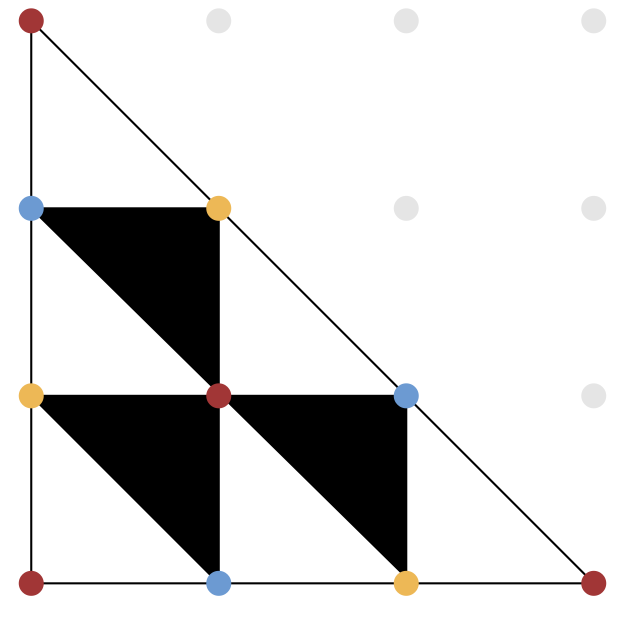
The signature $\sigma(\mathcal{T})$ of a balanced triangulation of a polygon is the absolute value of the difference of the number of white triangles and the number of the black triangles whose normalized volume is odd.

In [22]:
(foldable = T.FOLDABLE, signature = T.SIGNATURE)
Out[22]:
(foldable = true, signature = 3)

Now, a Wroński polynomial $W_{\mathcal{T},s}(x)$ has the lifted lattice points as exponents, and only one non-zero coefficient $c_i \in \mathbb{R}$ per color class of vertices of the triangulation $$W_{\mathcal{T},s}(x) = \sum_{i=0}^d c_i \left (\sum_{j:\;\textrm{color($a_j$)=$i$}} s^{\lambda_i} x^{a_j} \right ) \,.$$

A Wroński system consists of $d$ Wroński polynomials with respect to the same lattice points $A$ and lifting $\lambda$ such that for general $s = s_0 \in [0,1]$ it has precisely $d!\operatorname{vol}(\operatorname{conv}(A))$ distinct complex solutions, which is the highest possible number by Kushnirenko’s Theorem.

Soprunova and Sottile showed that a Wroński system has at least $\sigma(\mathcal{T})$ distinct real solutions if two conditions are satisfied.

1) A certain double cover of the real toric variety associated with $A$ must be orientable (this is the case here)

2) The Wroński center ideal, a zero-dimensional ideal in coordinates $x_1,x_2$ and $s$ depending on $\mathcal{T}$, has no real roots with $s$ coordinate between 0 and 1.

Goal: Verify condition 2) using HomotopyContinuation.jl.

Luckily, polymake already has an implementationof the Wroński center ideal

In [23]:
I = polytope.wronski_center_ideal(A, λ)
collect(I.GENERATORS)
Out[23]:
3-element Array{Polymake.Polynomial{Polymake.Rational,Int64},1}:
 pm::Polynomial<pm::Rational, long>
x_0^3*x_2^15 + x_0*x_1*x_2 + x_1^3 + x_2^12
 pm::Polynomial<pm::Rational, long>
x_0^2*x_2^9 + x_0*x_1^2 + x_1*x_2^3
 pm::Polynomial<pm::Rational, long>
x_0^2*x_1*x_2^5 + x_0*x_2^8 + x_1^2

We have to convert the ideal returned by Polymake.jl to a polynomial system which HomotopyContinuation.jl understands.

In [24]:
using HomotopyContinuation
# define a small helper function
function hc_poly(f, vars)
    M = Polymake.monomials_as_matrix(f)
    monomials = [prod(vars.^m) for m in eachrow(M)]
    coeffs = convert.(Int, Polymake.coefficients_as_vector(f))
    sum(map(*, coeffs, monomials))
end

@polyvar x[1:2] s;
HC_I = [hc_poly(f, [x;s]) for f in I.GENERATORS]
Out[24]:
3-element Array{DynamicPolynomials.Polynomial{true,Int64},1}:
 x₁³s¹⁵ + s¹² + x₁x₂s + x₂³
 x₁²s⁹ + x₂s³ + x₁x₂²
 x₁s⁸ + x₁²x₂s⁵ + x₂²

Since we are only interested in solutions in the algebraic torus $(\mathbb{C}^*)^3$ we can use a polyhedral homotopy to efficiently compute the solutions.

In [25]:
@time res = HomotopyContinuation.solve(HC_I; start_system = :polyhedral, only_torus = true)
┌ Warning: ProgressMeter by default refresh meters with additional information in IJulia via `IJulia.clear_output`, which clears all outputs in the cell. 
│  - To prevent this behaviour, do `ProgressMeter.ijulia_behavior(:append)`. 
│  - To disable this warning message, do `ProgressMeter.ijulia_behavior(:clear)`.
└ @ ProgressMeter /home/kalmar/.julia/packages/ProgressMeter/N86Uo/src/ProgressMeter.jl:441
Computing mixed cells... 3 	 Time: 0:00:00
  mixed_volume:  54
 61.383889 seconds (89.06 M allocations: 4.511 GiB, 4.38% gc time)
Out[25]:
Result{Array{Complex{Float64},1}} with 54 solutions
===================================================
• 54 non-singular solutions (2 real)
• 0 singular solutions (0 real)
• 54 paths tracked
• random seed: 562589

Out of the 54 complex roots only two solutions are real. Strictly speaking, this is here only checked heuristically by looking at the size of the imaginary parts.

In [26]:
HomotopyContinuation.real_solutions(res)
Out[26]:
2-element Array{Array{Float64,1},1}:
 [-0.21175800954334484, -215.72260079314532, 4.411470567441927]
 [-0.6943590430596771, -0.4142418845825889, -0.8952189506082182]

We see that no solution has the $s$-coordinate in $(0,1)$.

By Soprunova and Sottile result, the Wroński system with respect to $A$ and $\lambda$ for $s=1$ has at least $\sigma(\mathcal{T})=3$ real solutions. Let us verify this on an example.

In [27]:
c = Vector{Rational}[[19,8,-19], [39,7,42]]
W = polytope.wronski_system(A, λ, c, 1)
HC_W = [hc_poly(f, x) for f in W.GENERATORS]
Out[27]:
2-element Array{DynamicPolynomials.Polynomial{true,Int64},1}:
 19x₁³ - 19x₁²x₂ + 8x₁x₂² + 19x₂³ + 8x₁² + 19x₁x₂ - 19x₂² - 19x₁ + 8x₂ + 19
 39x₁³ + 42x₁²x₂ + 7x₁x₂² + 39x₂³ + 7x₁² + 39x₁x₂ + 42x₂² + 42x₁ + 7x₂ + 39
In [28]:
W_res = HomotopyContinuation.solve(HC_W)
Out[28]:
Result{Array{Complex{Float64},1}} with 9 solutions
==================================================
• 9 non-singular solutions (3 real)
• 0 singular solutions (0 real)
• 9 paths tracked
• random seed: 920847

Finally, we can use the ImplicitPlots.jl package to visualize the real solutions of the Wroński system W.

In [29]:
W_real = HomotopyContinuation.real_solutions(W_res)
using ImplicitPlots, Plots;
plt = plot(aspect_ratio = :equal);
implicit_plot!(plt, HC_W[1]);
implicit_plot!(plt, HC_W[2]; color=:indianred);
scatter!(first.(W_real), last.(W_real), markercolor=:black)
Out[29]:

Conclusion

  • Polymake.jl is a new interface to polymake with almost every polymake feature available
  • Seemless integration into Jupyter
  • Since Polymake.jl is in Julia this allows to easily combine polyhedral and numerical methods

Thank you for your attention